基础函数persp
persp函数
persp(x = seq(0, 1, length.out = nrow(z)),
      y = seq(0, 1, length.out = ncol(z)),
      z, xlim = range(x), ylim = range(y),
      zlim = range(z, na.rm = TRUE),
      xlab = NULL, ylab = NULL, zlab = NULL,
      main = NULL, sub = NULL,
      theta = 0, phi = 15, r = sqrt(3), d = 1,
      scale = TRUE, expand = 1,
      col = "white", border = NULL, ltheta = -135, lphi = 0,
      shade = NA, box = TRUE, axes = TRUE, nticks = 5,
      ticktype = "simple", ...)
- 参数x和y分别是两个数值向量,z是一个与前两个参数对应的矩阵
- xlim、ylim和zlim分别设定三个坐标轴的范围
- xlab、ylab和zlab分别设定三个坐标轴的标题
- theta和phi分别设定立体图形左右方向和上下方向旋转的角度
- r设定眼睛离透视图中心的距离,这个距离的远近会给我们一种从远近看物体的感觉
- d设定立体效果的程度,大于1的值会减弱立体程度,反之会增强立体程度
- scale为逻辑值,决定是否对三个坐标进行缩放,若为TRUE,则x、y和z都会被缩放到[0, 1]范围内,若为FALSE,那么所有坐标轴都按照数据的原始量纲处理,这样可以得到数据的真实比例
- expand为z轴的缩放因子,它决定了z轴的长短
- col为组成曲面的所有小方块的颜色;border为组成曲面的小方块的边框样式,设置为NA可以去掉边 框
- ltheta和lphi设置透视图的光源位置
- shade决定的阴影效果;box为逻辑值,设定透视图是否需要画外框
- axes决定是否画坐标轴;nticks为坐标轴刻度线的数目;ticktype设定坐标轴刻度类型,取值’simple’则简单画箭头表示坐标轴,’detailed’则将详细的刻度标记在坐标轴上
实例
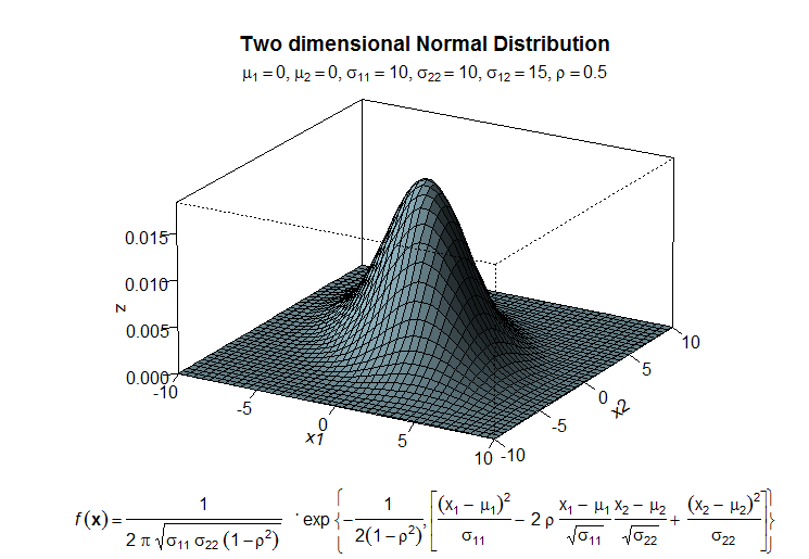
这里我们使用persp函数来展示一下二维正态分布密度函数图。 二维正态分布密度函数的公式:
mu1<-0 # setting the expected value of x1
mu2<-0 # setting the expected value of x2
s11<-10 # setting the variance of x1
s12<-15 # setting the covariance between x1 and x2
s22<-10 # setting the variance of x2
rho<-0.5 # setting the correlation coefficient between x1 and x2
x1<-seq(-10,10,length=41) # generating the vector series x1
x2<-x1 # copying x1 to x2

f<-function(x1,x2)
{
term1<-1/(2*pi*sqrt(s11*s22*(1-rho^2)))
term2<--1/(2*(1-rho^2))
term3<-(x1-mu1)^2/s11
term4<-(x2-mu2)^2/s22
term5<--2*rho*((x1-mu1)*(x2-mu2))/(sqrt(s11)*sqrt(s22))

term1*exp(term2*(term3+term4-term5))
} # setting up the function of the multivariate normal density
#
z<-outer(x1,x2,f) # calculating the density values
#
persp(x1, x2, z,
main="Two dimensional Normal Distribution",
sub=expression(italic(f)~(bold(x))==frac(1,2~pi~sqrt(sigma[11]~
sigma[22]~(1-rho^2)))~phantom(0)^bold(.)~exp~bgroup("{",
list(-frac(1,2(1-rho^2)),
bgroup("[", frac((x[1]~-~mu[1])^2, sigma[11])~-~2~rho~frac(x[1]~-~mu[1],
sqrt(sigma[11]))~ frac(x[2]~-~mu[2],sqrt(sigma[22]))~+~
frac((x[2]~-~mu[2])^2, sigma[22]),"]")),"}")),
col="lightblue",
theta=30, phi=20,
r=50,
d=0.1,
expand=0.5,
ltheta=90, lphi=180,
shade=0.75,
ticktype="detailed",
nticks=5) # produces the 3-D plot
#
mtext(expression(list(mu[1]==0,mu[2]==0,sigma[11]==10,sigma[22]==10,sigma[12
]==15,rho==0.5)), side=3) # adding a text line to the graph
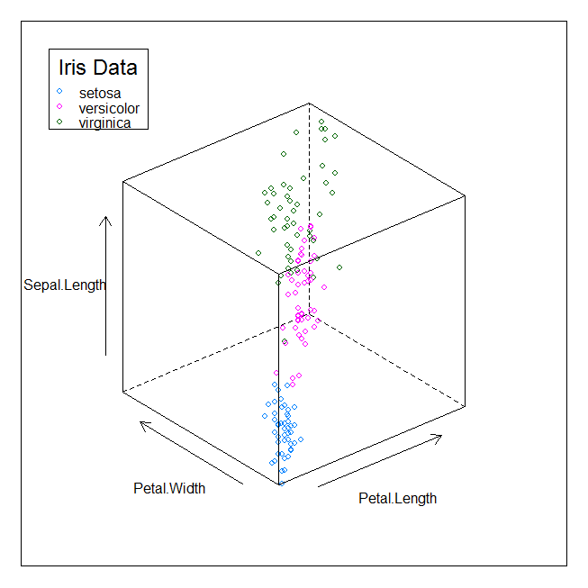
lattice包的函数
library(lattice)
data(iris)
cloud(Sepal.Length ~ Petal.Length * Petal.Width, data = iris,
groups = Species,
perspective = FALSE,
key = list(title = "Iris Data", x = .05, y=.95, border = TRUE,
points = Rows(trellis.par.get("superpose.symbol"), 1:3),
text = list(levels(iris$Species))))
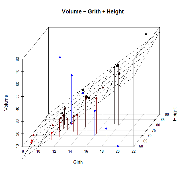
scatterplot3d包的函数
scatterplot3d包主要包含三个函数,其中:
- scatterplotplot3d函数为包scatterplot3d的基础函数,能够打开画图,画出点或线
- points3d向用函数scatterplotplot3d画好的图上添加点或线
- plane3d向用函数scatterplotplot3d画好的图上添加趋势面
library(scatterplot3d)
data(trees)
s3d <- scatterplot3d(trees, type="h", highlight.3d=TRUE,
angle=55, scale.y=0.7, pch=16, main="Volume ~ Grith + Height")
# Now adding some points to the "scatterplot3d"
s3d$points3d(seq(10,20,2), seq(85,60,-5), seq(60,10,-10),
col="blue", type="h", pch=16)
# Now adding a regression plane to the "scatterplot3d"
attach(trees)
my.lm <- lm(Volume ~ Girth + Height)
s3d$plane3d(my.lm)
rgl包的函数
利用rgl包作出的三维图像,可以通过鼠标调整不同的角度。
library(rgl)
plot3d(1:5,1:5, z = c(10, 20, 30, 40, 70), col="red", size=5)
# save image
rgl.snapshot('plot1.png')
rgl.postscript("plot1.pdf", "pdf", drawText = TRUE)
  r3dDefaults
    open3d()
    shade3d(cube3d(color = rep(rainbow(6), rep(4, 6))))
	rgl.snapshot('plot2.png')
rgl.postscript("plot2.pdf", "pdf", drawText = TRUE)
    save <- par3d(userMatrix = rotationMatrix(90*pi/180, 1, 0, 0))
    save
    par3d("userMatrix")
    par3d(save)
    par3d("userMatrix")
话外篇
下面的部分与文章主题没有关系,只是记述一下hexo中数学公式的表示方式。